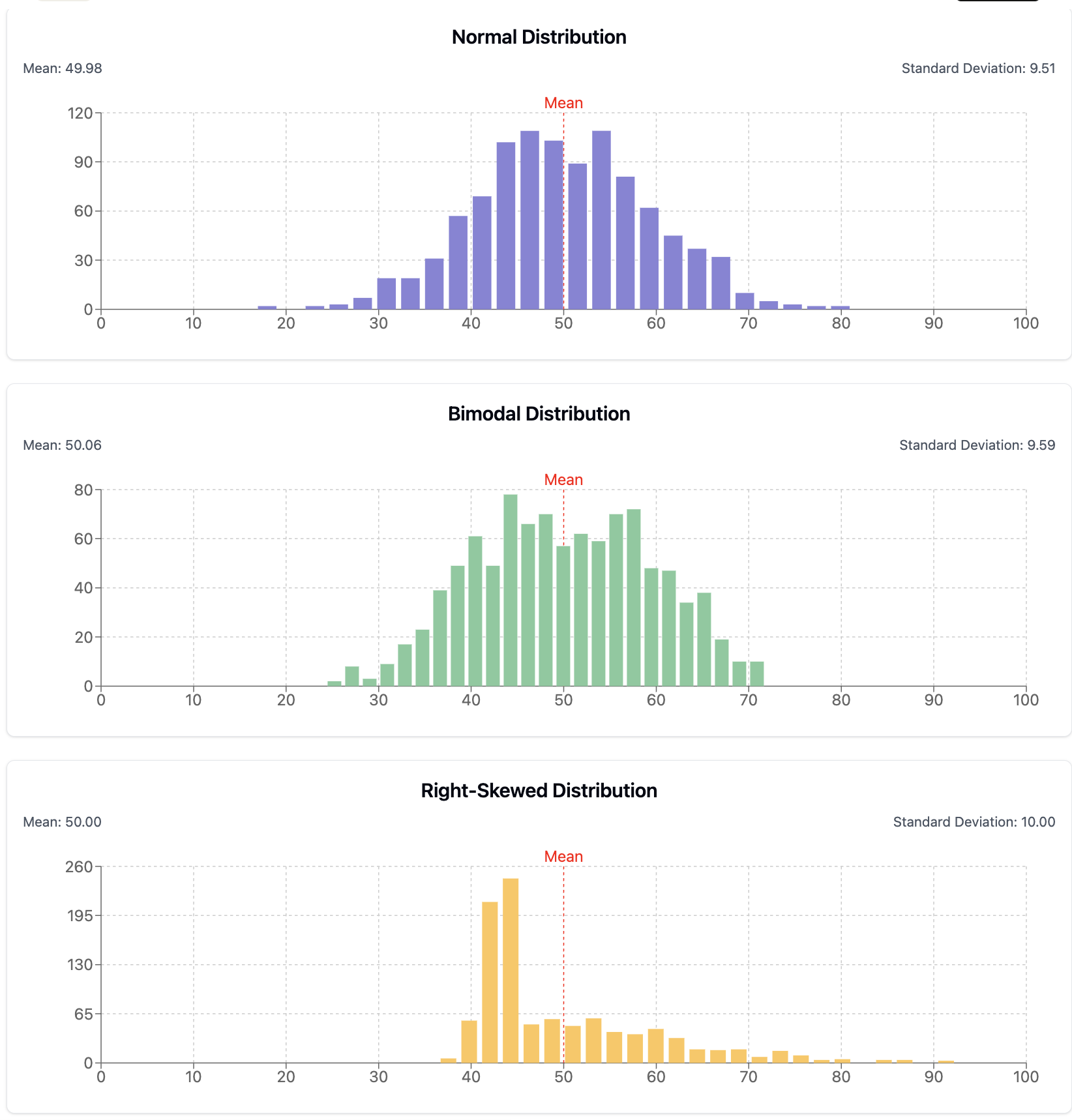
For a highly skewed distribution of housing prices in a city, which measure of central tendency would be MOST appropriate to report?
Mean (average) price
The mean is highly influenced by extreme values and can be misleading for skewed distributions. In housing prices, a few very expensive properties can pull the mean upward, making it unrepresentative of typical prices.
Median price
Correct! The median is the most appropriate measure for skewed distributions like housing prices because it’s not influenced by extreme values. It represents the middle value, giving a better sense of the "typical" home price.
Modal price (most common price)
While the mode can be useful for categorical data, it’s generally less informative for continuous variables like housing prices, which may not have many exact repeated values.
Midrange (average of minimum and maximum prices)
The midrange is highly influenced by outliers and would be particularly problematic for a skewed distribution of housing prices, where the maximum value could be dramatically higher than most values.
Activity21.Calculating Summary Statistics in CODAP.
In this activity, you’ll calculate and interpret summary statistics for your dataset.
(a)
Select at least three numerical variables from your dataset. For each variable, use CODAP to calculate:
Mean, median, and mode
Standard deviation and interquartile range
Minimum, maximum, and range
(b)
Create visualizations (histograms or box plots) for each variable and examine how the summary statistics relate to the distribution shape.
(c)
For each variable, determine which measure of central tendency (mean, median, or mode) best represents the "typical" value and explain why.
(d)
Calculate correlation coefficients between pairs of numerical variables. Identify the strongest positive and negative correlations in your dataset.
SubsectionCreating Derived Variables
Often, the variables we need for analysis aren’t directly present in our original dataset. Creating derived variables allows us to transform existing data into more meaningful measures.
Common types of derived variables include:
Mathematical Transformations
Logarithmic transformations to handle skewed data
Standardization (z-scores) to compare different scales
Unit conversions (e.g., meters to feet, Celsius to Fahrenheit)
Combinations of Variables
Ratios and proportions (e.g., debt-to-income ratio)
Indices combining multiple measures (e.g., air quality index)
Weighted averages (e.g., GPA calculation)
Categorical Derivations
Binning numerical variables into categories (e.g., age groups)
Creating binary indicators (e.g., high-risk vs. low-risk)
Recoding categorical variables (e.g., combining similar categories)
Temporal Derivations
Calculating time differences (e.g., days between events)
In this activity, you’ll create and analyze derived variables in your dataset.
(a)
Create at least three derived variables in your dataset, including:
A mathematical transformation of an existing variable (e.g., log, square root, or standardization)
A ratio or relationship between two variables
A categorical variable derived from a numerical variable (e.g., binning into groups)
(b)
Create visualizations showing the relationships between your original variables and the derived variables.
(c)
Explore how your derived variables relate to other variables in the dataset. Do they reveal patterns that weren’t obvious with the original variables?
SubsectionGrouping and Aggregation Techniques
Grouping and aggregation allow us to summarize data at different levels and examine patterns across categories. These techniques help us answer questions about how metrics vary between groups.
Common grouping and aggregation operations include:
Group By
Dividing data into subsets based on categories (e.g., by region, income level, or time period).
Aggregate Functions
Calculating summary statistics for each group:
Count: Number of observations
Sum: Total of values
Average: Mean value
Min/Max: Smallest/largest values
Standard Deviation: Measure of spread
Pivot Tables
Reorganizing data to show aggregated values across multiple dimensions.
Hierarchical Grouping
Nesting groups within groups (e.g., neighborhoods within districts within cities).
Example74.Grouping in Community Health Analysis.
In our Community Health dataset, we might use grouping and aggregation to:
Calculate average asthma rates by income quartile to examine socioeconomic health disparities
Compare environmental quality metrics across different regions of the city
Examine how multiple health indicators vary across neighborhoods with different levels of green space access
Create a pivot table showing average health metrics by both region and income level simultaneously
Calculate the standard deviation of air quality within each region to understand environmental variability
Checkpoint75.Purpose of Grouping and Aggregation.
What is the PRIMARY purpose of grouping and aggregation in data analysis?
To remove outliers from a dataset
While aggregation may reduce the impact of outliers in summary statistics, this is not the primary purpose of grouping and aggregation.
To understand patterns and variations across categories or subsets
Correct! The primary purpose of grouping and aggregation is to reveal how metrics and patterns vary across different categories or subsets, allowing for meaningful comparisons.
To reduce the size of large datasets
While aggregation does create a more compact summary, this is a side effect rather than the primary purpose of grouping and aggregation.
To correct errors in the original data
Grouping and aggregation do not correct errors in the original data; in fact, they might obscure some errors by combining them with correct values.
Activity23.Grouping and Aggregation in CODAP.
In this activity, you’ll practice grouping and aggregating data in CODAP.
(a)
Identify at least two categorical variables in your dataset that would be meaningful to group by.
(b)
For each grouping variable, create a summary table in CODAP that shows aggregated measures (mean, count, etc.) of at least two numerical variables for each group.
(c)
Create visualizations comparing these groups. Use bar charts or box plots to show how the numerical variables differ across categories.
(d)
Try creating a two-way grouping by two different categorical variables. Examine how this more detailed breakdown reveals patterns that might not be apparent in single-variable groupings.